Suicide
suicide_df =
  read_excel(
    "./data/suicide_data.xlsx",
    sheet = 1,
    col_names = TRUE) %>%
  janitor::clean_names() %>%
  mutate(
    population = (suicide_no / suicide_100k) * 100000,
    sex = as.factor(sex),
    age = as.factor(age)
  )

average_20years = sum(suicide_df$suicide_no) / sum(suicide_df$population) * 100000

suicide_state_df =
  read_excel(
    "./data/suicide_data.xlsx",
    sheet = 2,
    range = "A1:D351",
    skip = 1,
    col_names = TRUE) %>%
  janitor::clean_names() %>%
  rename(
     suicide_no = deaths,
     suicide_100k = death_rate) %>%
  mutate(
    population = (suicide_no / suicide_100k) * 100000
  )

suicide_means_df =
   read_excel(
    "./data/suicide_data.xlsx",
    sheet = 3,
    col_names = TRUE) %>%
  janitor::clean_names() %>%
  pivot_longer(
    firearm:others,
    names_to = "means",
    values_to = "rate"
  ) %>%
  mutate(
       sex = as.factor(sex),
       means = as.factor(means))
National Trend (2000-2020)
The US national suicide rates increase from 2000 to 2018, then decline from 2018 to 2020. The average suicide rate from 2000 to 2020 is 14.2 per 100,000 (represented with red dot line).
suicide_plot = suicide_df %>%
  group_by(year) %>%
  summarize(
    population = sum(population),
    suicide = sum(suicide_no),
    suicide_100k = (suicide / population) * 100000
  ) %>%
  ggplot(aes(x = year, y = suicide_100k)) +
  geom_line(col = "deepskyblue", size = 1) +
  geom_point(col = "deepskyblue", size = 2) +
  geom_hline(
    yintercept = average_20years, linetype = 2, color = "red", size = 1) +
  scale_x_continuous(breaks = seq(2000, 2020, 5)) +
  scale_y_continuous(breaks = seq(8, 18, 1)) +
  labs(title = "US National Suicide Rate (per 100K), 2000-2020",
       x = "Year",
       y = "Suicides per 100k")

ggplotly(suicide_plot)
State Level
Cumulative Suicide Rate
Wyoming has the highest suicide rate and New Jersey has the lowest suicide rate from 2014-2020. The top 5 states with high cumulative suicide rates are Wyoming, Alaska, Montana, New Mexico, and Idaho; the top 5 states with low cumulative suicide rates are New Jersey, New York, Massachusetts, Maryland and Connecticut.
suicide_state_df %>%
  group_by(state) %>%
  summarize(
    population = sum(population),
    suicide = sum(suicide_no),
    suicide_100k = (suicide / population) * 100000
  ) %>%
  mutate(
    state = fct_reorder(state, suicide_100k)) %>%
  ggplot(aes(x = suicide_100k, y = state, fill = state )) +
  geom_bar(stat = "identity") +
  scale_x_continuous(breaks = seq(0, 30, 2)) +
  labs(
    title = "Cumulative Suicide Rate, by State, 2014-2020",
    x = "Suicides per 100k",
    y = "State") +
  theme(legend.position = "right")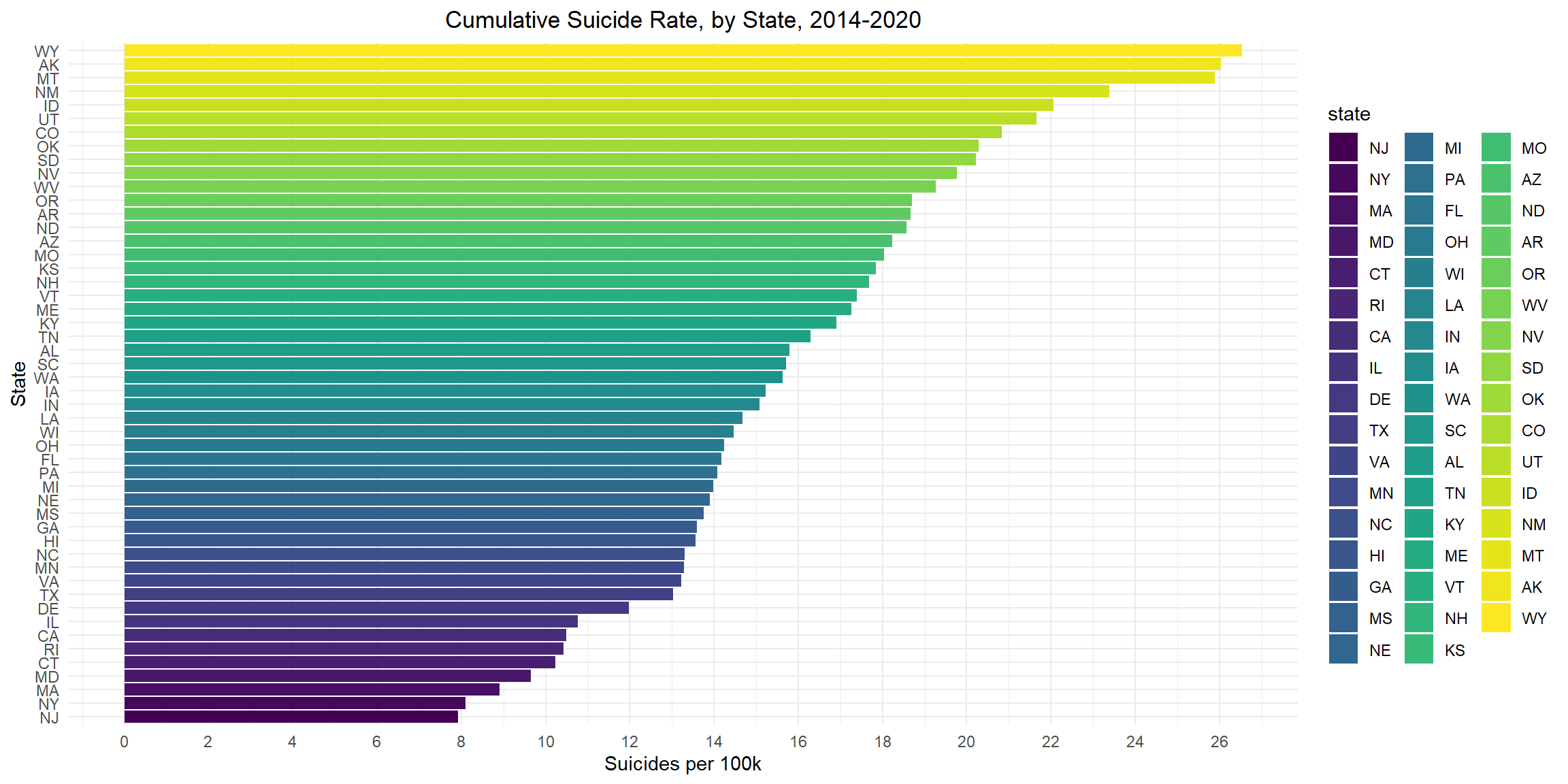
Suicide Rate
Between 2014 and 2020, the state with the largest change in suicide rate is Wyoming, from 20.6 to 30.5; the state with the smallest change in suicide rate is New York, from 7.8 to 8.3.
suicide_state_df %>%
  ggplot(aes(x = suicide_100k, y = state, color = year)) +
  geom_line(size = 1) +
  geom_point(size = 2) +
  labs(
    title = "Suicide Rate for Each State Over Years, 2014-2020",
    x = "State",
    y = "Suicides per 100K") +
  theme(legend.position = "right")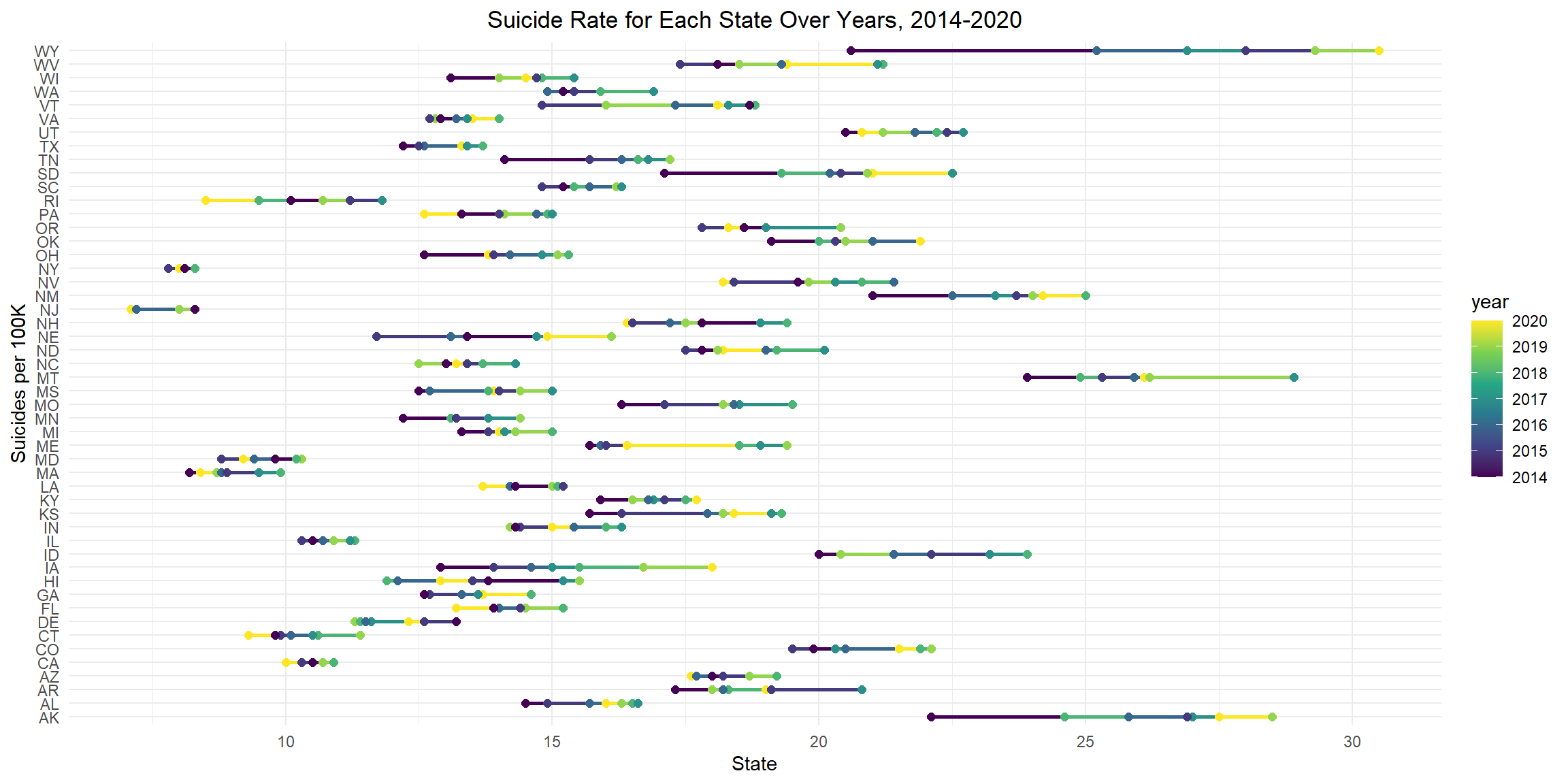
Sex, Age, Combination
Sex
Nationally, the overall suicide rate for males is about 4 times that of females. For females, suicide rates peak in 2018 and decline since then; for males, suicide rates peak in 2017 and decline since then. From year 2000 to 2020, the male suicide rate remains apparently higher than the female suicide rate, and the ratio is constantly about 4:1.
total_sex_plot = suicide_df %>%
  group_by(sex) %>%
  summarize(
    population = sum(population),
    suicide = sum(suicide_no),
    suicide_100k = (suicide / population) * 100000
  ) %>%
  ggplot(aes(x = sex, y = suicide_100k, fill = sex )) +
  geom_bar(stat = "identity") +
  scale_y_continuous(breaks = seq(0, 24, 4)) +
  labs(
    title = "National Suicide Rate, by Sex",
    x = "Sex",
    y = "Suicides per 100k")


year_sex_plot = suicide_df %>%
  group_by(year, sex) %>%
  summarize(
    population = sum(population),
    suicide = sum(suicide_no),
    suicide_100k = (suicide / population) * 100000
  ) %>%
  ggplot(aes(x = year, y = suicide_100k, color = sex)) +
  geom_line(size = 1) +
  geom_point(size = 2) +
  scale_y_continuous(breaks = seq(0, 30, 5)) +
  labs(
    title = "Suicide Trend Over Years, by Sex",
    x = "Year",
    y = "Suicides per 100k"
  )

grid.arrange(total_sex_plot, year_sex_plot, ncol = 2 )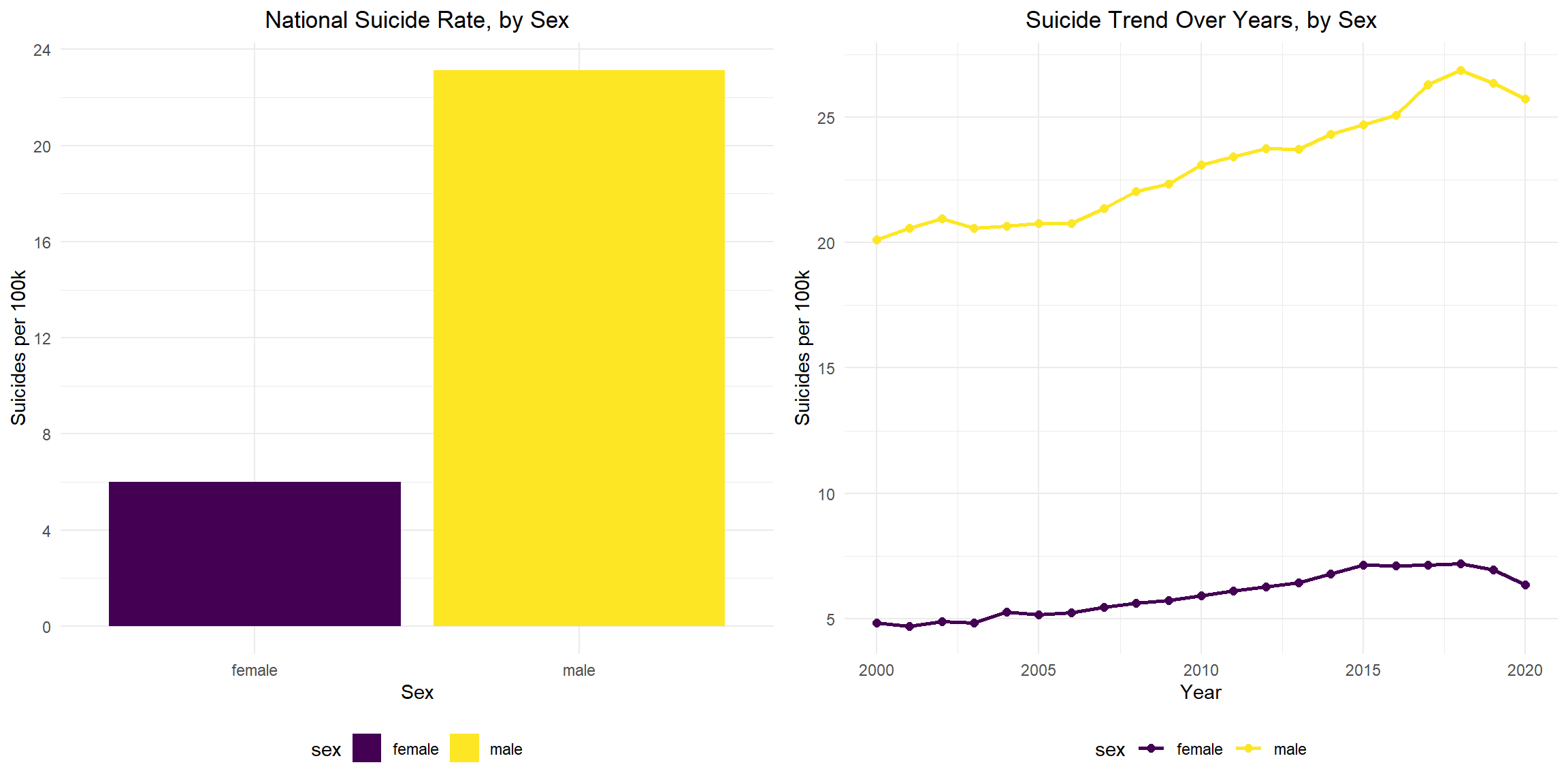
Age
Nationally, aged 45-64 had the highest suicide rate, second highest group is aged 75+. The 10-14 aged group has the lowest suicide rate. From year 2000 to 2020, the suicide rate of group aged 10-14 remains roughly static and small. Suicide rates in all other age groups show an overall upward trend. Among them, the group aged 25-44 has the largest change, roughly from 10 to 18 suicide rate per 100k. The suicide rates of those aged 45-64 and aged 65-74 start to drop since 2018.
total_age_plot = suicide_df %>%
  group_by(age) %>%
  summarize(
    population = sum(population),
    suicide = sum(suicide_no),
    suicide_100k = (suicide / population) * 100000
  ) %>%
  ggplot(aes(x = age, y = suicide_100k, fill = age )) +
  geom_bar(stat = "identity") +
  scale_y_continuous(breaks = seq(0, 20, 2)) +
  labs(
    title = "National Suicide Rate, by Age",
    x = "Age",
    y = "Suicides per 100k")


year_age_plot = suicide_df %>%
  group_by(year, age) %>%
  summarize(
    population = sum(population),
    suicide = sum(suicide_no),
    suicide_100k = (suicide / population) * 100000
  ) %>%
  ggplot(aes(x = year, y = suicide_100k,  color = age)) +
  geom_line(size = 1) +
  geom_point(size = 2) +
  scale_y_continuous(breaks = seq(0, 24, 2)) +
  labs(
    title = "Suicide Trend Over Years, by Age",
    x = "Year",
    y = "Suicides per 100k"
  )

grid.arrange(total_age_plot, year_age_plot, ncol = 2 )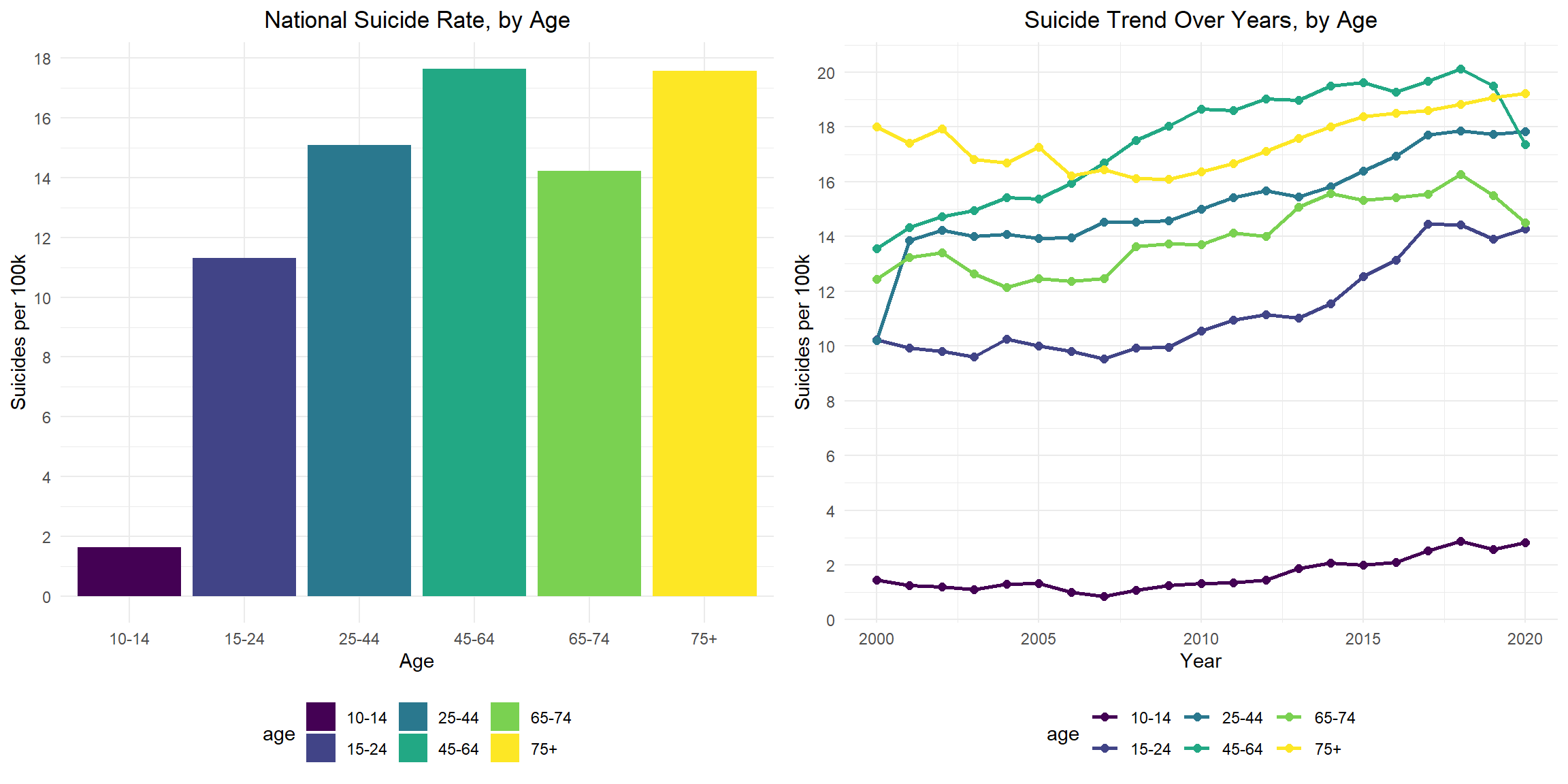
Sex and Age
- Suicide Rate for Females, by Age Group, 2000-2020
Recently (from 2018 to 2020), suicide rates decrease in females aged 25-44, 45-64, 65-74 and 75+, but increase for those aged 15-24 and keep constant for those aged 10-14. Suicide rates are highest for those females aged 45-64 over the period of 2000-2020. The suicide rates increase from 6.2 in 2000 to the highest 10.2 in 2015, and then decline to 7.9 in 2020. Suicide rates are consistently lowest for those females aged 10-14 over the period of 2000-2020. The suicide rates increase from 0.6 in 2000 to the highest 2.0 in 2018, and then keep constant through 2020.But the rate more than triples from 0.6 (2000) to 2.0 (2020). The suicide rates of those aged 75+ are relatively stable between 2000 and 2020.
female_plot = suicide_df %>%
  filter(sex == "female") %>%
  group_by(year, age) %>%
  summarize(
    population = sum(population),
    suicide = sum(suicide_no),
    suicide_100k = (suicide / population) * 100000
  ) %>%
  ggplot(aes(x = year, y = suicide_100k,  color = age)) +
  geom_line(size = 1) +
  geom_point(size = 2) +
  scale_y_continuous(breaks = seq(0, 12, 2)) +
  labs(
    title = "Suicide Trend  for Females by Age, 2000-2020",
    x = "Year",
    y = "Suicides per 100k"
  )

ggplotly(female_plot)- Suicide Rate for Males, by Age Group, 2000-2020
Recently (from 2018 to 2020), suicide rates decrease in males aged 45-64 and 65-74, but increase for those aged 10-14, 15-24, 25-44 and 75+. Suicide rates are consistently highest for those males aged 75+ over the period of 2000-2020. The suicide rate decline from highest 42.4 in 2000 to the lowest 35.6 in 2009, and then increase to 40.5 in 2020. Suicide rates are consistently lowest for those males aged 10-14 over the period of 2000-2020. The suicide rate declines from 2.3 in 2000 to 1.2 in 2007, and then increase to 3.6 in 2020. The suicide rates of those aged 10-14 are relatively stable between 2000 and 2020.
male_plot =  suicide_df %>%
  filter(sex == "male") %>%
  group_by(year, age) %>%
  summarize(
    population = sum(population),
    suicide = sum(suicide_no),
    suicide_100k = (suicide / population) * 100000
  ) %>%
  ggplot(aes(x = year, y = suicide_100k,  color = age)) +
  geom_line(size = 1) +
  geom_point(size = 2) +
  scale_y_continuous(breaks = seq(0, 45, 5)) +
  labs(
    title = "Suicide Trend  for Males by Age, 2000-2020",
    x = "Year",
    y = "Suicides per 100k"
  )

ggplotly(male_plot)
Sex and Means of Suicide
Suicide Rate for Females, by Means of Suicide, 2000-2020
For females, the rates for firearm-related suicide increase from 1.4 in 2008 to 1.9 in 2016 and remain stable through 2020. Suicides by firearm become the leading means for females in 2020. The rates for poisoning-related suicide increase from 1.4 in 2000 to 2.0 in 2015 and decline to 1.5 in 2020. Before 2016, poisoning-related suicides are the leading means for females. The rates for suffocation-related suicides dramatically increase from 0.7 in 2000 to 1.9 in 2018, and then decline slightly to 1.7 in 2020. Overall, the rates are more than doubled over the study period. During the study period, differences in rates for suicide by firearm, poisoning and suffocation decline. In 2020, females have the highest rate for firearm suicide (1.8), followed by suffocation (1.7) and poisoning (1.5).
female_means_plot = suicide_means_df %>%
  filter(sex == "female") %>%
  ggplot(aes(x = year, y = rate,  color = means)) +
  geom_line(size = 1) +
  geom_point(size = 2) +
  scale_y_continuous(breaks = seq(0, 2.5, 0.5)) +
  labs(
    title = "Female Suicide Rates, by Means of Suicide, 2000-2020",
    x = "Year",
    y = "Suicides per 100k"
  )

ggplotly(female_means_plot)
Suicide Rate for Males, by Means of Suicide, 2000-2020
For males, the rates for firearm-related suicide decline from 11.0 in 2000 to 10.3 in 2006 and then increase to 12.5 in 2020. The rates for firearm-related suicide are much higher than that for all other suicide means (poisoning, suffocation and others). Overall, the rates for poisoning-related suicide decline from 2.1 in 2000 to 1.7 in 2020. And the rates remain in a relatively low level. The rates for suffocation-related suicides increase from 3.4 in 2000 to 6.7 in 2018, and then decline to 6.1 in 2020. Overall, the rates are almost doubled during the study period. During the study period, the difference in rates for firearm-related suicide and suffocation-related suicide narrows, but the difference in rates for suffocation-related suicide and poisoning-related suicide widens. For the same suicide means, the rates for males are generally higher than that of females.
male_means_plot = suicide_means_df %>%
  filter(sex == "male") %>%
  ggplot(aes(x = year, y = rate,  color = means)) +
  geom_line(size = 1) +
  geom_point(size = 2) +
  scale_y_continuous(breaks = seq(0, 16, 2)) +
  labs(
    title = "Male Suicide Rates, by Means of Suicide, 2000-2020",
    x = "Year",
    y = "Suicides per 100k"
  )

ggplotly(male_means_plot)
Conclusion
- The US national suicide rates increase from 2000 to 2018, then decline from 2018 to 2020.
- The suicide rates are high in the US overall, with variations between states and over years. Wyoming has the highest suicide rate and New Jersey has the lowest suicide rate from 2014-2020.
- For both females and males, suicide rates are lower in 2020 than in 2018 and 2019. Overall, the suicide rate for males is much higher than that of females.
- Overall, suicide rates increase with age (except age group 65-74). Suicide rates in all age groups shown an upward trend.
- The leading means of suicide for females in 2020 is firearm-related, before 2017, poisoning-related is the leading means. The leading means of suicide for males is firearm-related over 20 years.